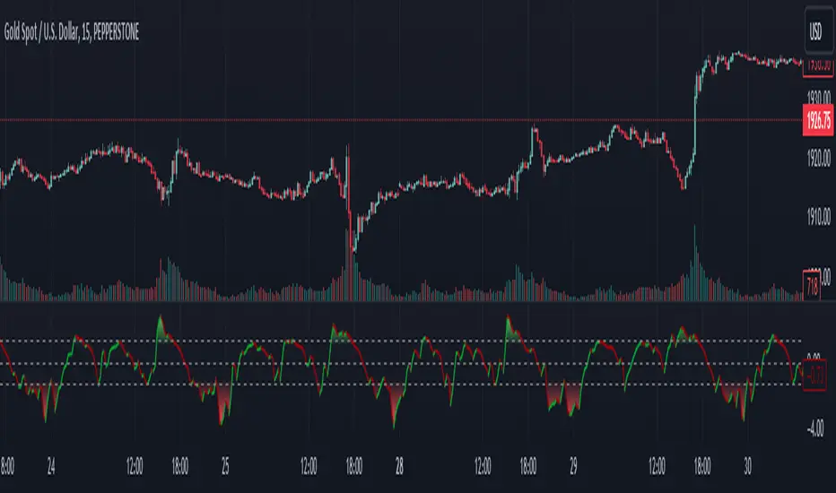
MERV: Market Entropy & Rhythm Visualizer [BullByte]The MERV (Market Entropy & Rhythm Visualizer) indicator analyzes market conditions by measuring entropy (randomness vs. trend), tradeability (volatility/momentum), and cyclical rhythm. It provides traders with an easy-to-read dashboard and oscillator to understand when markets are structured or choppy, and when trading conditions are optimal.
Purpose of the Indicator
MERV’s goal is to help traders identify different market regimes. It quantifies how structured or random recent price action is (entropy), how strong and volatile the movement is (tradeability), and whether a repeating cycle exists. By visualizing these together, MERV highlights trending vs. choppy environments and flags when conditions are favorable for entering trades. For example, a low entropy value means prices are following a clear trend line, whereas high entropy indicates a lot of noise or sideways action. The indicator’s combination of measures is original: it fuses statistical trend-fit (entropy), volatility trends (ATR and slope), and cycle analysis to give a comprehensive view of market behavior.
Why a Trader Should Use It
Traders often need to know when a market trend is reliable vs. when it is just noise. MERV helps in several ways: it shows when the market has a strong direction (low entropy, high tradeability) and when it’s ranging (high entropy). This can prevent entering trend-following strategies during choppy periods, or help catch breakouts early. The “Optimal Regime” marker (a star) highlights moments when entropy is very low and tradeability is very high, typically the best conditions for trend trades. By using MERV, a trader gains an empirical “go/no-go” signal based on price history, rather than guessing from price alone. It’s also adaptable: you can apply it to stocks, forex, crypto, etc., on any timeframe. For example, during a bullish phase of a stock, MERV will turn green (Trending Mode) and often show a star, signaling good follow-through. If the market later grinds sideways, MERV will shift to magenta (Choppy Mode), warning you that trend-following is now risky.
Why These Components Were Chosen
Market Entropy (via R²) : This measures how well recent prices fit a straight line. We compute a linear regression on the last len_entropy bars and calculate R². Entropy = 1 - R², so entropy is low when prices follow a trend (R² near 1) and high when price action is erratic (R² near 0). This single number captures trend strength vs noise.
Tradeability (ATR + Slope) : We combine two familiar measures: the Average True Range (ATR) (normalized by price) and the absolute slope of the regression line (scaled by ATR). Together they reflect how active and directional the market is. A high ATR or strong slope means big moves, making a trend more “tradeable.” We take a simple average of the normalized ATR and slope to get tradeability_raw. Then we convert it to a percentile rank over the lookback window so it’s stable between 0 and 1.
Percentile Ranks : To make entropy and tradeability values easy to interpret, we convert each to a 0–100 rank based on the past len_entropy periods. This turns raw metrics into a consistent scale. (For example, an entropy rank of 90 means current entropy is higher than 90% of recent values.) We then divide by 100 to plot them on a 0–1 scale.
Market Mode (Regime) : Based on those ranks, MERV classifies the market:
Trending (Green) : Low entropy rank (<40%) and high tradeability rank (>60%). This means the market is structurally trending with high activity.
Choppy (Magenta) : High entropy rank (>60%) and low tradeability rank (<40%). This is a mostly random, low-momentum market.
Neutral (Cyan) : All other cases. This covers mixed regimes not strongly trending or choppy.
The mode is shown as a colored bar at the bottom: green for trending, magenta for choppy, cyan for neutral.
Optimal Regime Signal : Separately, we mark an “optimal” condition when entropy_norm < 0.3 and tradeability > 0.7 (both normalized 0–1). When this is true, a ★ star appears on the bottom line. This star is colored white when truly optimal, gold when only tradeability is high (but entropy not quite low enough), and black when neither condition holds. This gives a quick visual cue for very favorable conditions.
What Makes MERV Stand Out
Holistic View : Unlike a single-oscillator, MERV combines trend, volatility, and cycle analysis in one tool. This multi-faceted approach is unique.
Visual Dashboard : The fixed on-chart dashboard (shown at your chosen corner) summarizes all metrics in bar/gauge form. Even a non-technical user can glance at it: more “█” blocks = a higher value, colors match the plots. This is more intuitive than raw numbers.
Adaptive Thresholds : Using percentile ranks means MERV auto-adjusts to each market’s character, rather than requiring fixed thresholds.
Cycle Insight : The rhythm plot adds information rarely found in indicators – it shows if there’s a repeating cycle (and its period in bars) and how strong it is. This can hint at natural bounce or reversal intervals.
Modern Look : The neon color scheme and glow effects make the lines easy to distinguish (blue/pink for entropy, green/orange for tradeability, etc.) and the filled area between them highlights when one dominates the other.
Recommended Timeframes
MERV can be applied to any timeframe, but it will be more reliable on higher timeframes. The default len_entropy = 50 and len_rhythm = 30 mean we use 30–50 bars of history, so on a daily chart that’s ~2–3 months of data; on a 1-hour chart it’s about 2–3 days. In practice:
Swing/Position traders might prefer Daily or 4H charts, where the calculations smooth out small noise. Entropy and cycles are more meaningful on longer trends.
Day trader s could use 15m or 1H charts if they adjust the inputs (e.g. shorter windows). This provides more sensitivity to intraday cycles.
Scalpers might find MERV too “slow” unless input lengths are set very low.
In summary, the indicator works anywhere, but the defaults are tuned for capturing medium-term trends. Users can adjust len_entropy and len_rhythm to match their chart’s volatility. The dashboard position can also be moved (top-left, bottom-right, etc.) so it doesn’t cover important chart areas.
How the Scoring/Logic Works (Step-by-Step)
Compute Entropy : A linear regression line is fit to the last len_entropy closes. We compute R² (goodness of fit). Entropy = 1 – R². So a strong straight-line trend gives low entropy; a flat/noisy set of points gives high entropy.
Compute Tradeability : We get ATR over len_entropy bars, normalize it by price (so it’s a fraction of price). We also calculate the regression slope (difference between the predicted close and last close). We scale |slope| by ATR to get a dimensionless measure. We average these (ATR% and slope%) to get tradeability_raw. This represents how big and directional price moves are.
Convert to Percentiles : Each new entropy and tradeability value is inserted into a rolling array of the last 50 values. We then compute the percentile rank of the current value in that array (0–100%) using a simple loop. This tells us where the current bar stands relative to history. We then divide by 100 to plot on .
Determine Modes and Signal : Based on these normalized metrics: if entropy < 0.4 and tradeability > 0.6 (40% and 60% thresholds), we set mode = Trending (1). If entropy > 0.6 and tradeability < 0.4, mode = Choppy (-1). Otherwise mode = Neutral (0). Separately, if entropy_norm < 0.3 and tradeability > 0.7, we set an optimal flag. These conditions trigger the colored mode bars and the star line.
Rhythm Detection : Every bar, if we have enough data, we take the last len_rhythm closes and compute the mean and standard deviation. Then for lags from 5 up to len_rhythm, we calculate a normalized autocorrelation coefficient. We track the lag that gives the maximum correlation (best match). This “best lag” divided by len_rhythm is plotted (a value between 0 and 1). Its color changes with the correlation strength. We also smooth the best correlation value over 5 bars to plot as “Cycle Strength” (also 0 to 1). This shows if there is a consistent cycle length in recent price action.
Heatmap (Optional) : The background color behind the oscillator panel can change with entropy. If “Neon Rainbow” style is on, low entropy is blue and high entropy is pink (via a custom color function), otherwise a classic green-to-red gradient can be used. This visually reinforces the entropy value.
Volume Regime (Dashboard Only) : We compute vol_norm = volume / sma(volume, len_entropy). If this is above 1.5, it’s considered high volume (neon orange); below 0.7 is low (blue); otherwise normal (green). The dashboard shows this as a bar gauge and percentage. This is for context only.
Oscillator Plot – How to Read It
The main panel (oscillator) has multiple colored lines on a 0–1 vertical scale, with horizontal markers at 0.2 (Low), 0.5 (Mid), and 0.8 (High). Here’s each element:
Entropy Line (Blue→Pink) : This line (and its glow) shows normalized entropy (0 = very low, 1 = very high). It is blue/green when entropy is low (strong trend) and pink/purple when entropy is high (choppy). A value near 0.0 (below 0.2 line) indicates a very well-defined trend. A value near 1.0 (above 0.8 line) means the market is very random. Watch for it dipping near 0: that suggests a strong trend has formed.
Tradeability Line (Green→Yellow) : This represents normalized tradeability. It is colored bright green when tradeability is low, transitioning to yellow as tradeability increases. Higher values (approaching 1) mean big moves and strong slopes. Typically in a market rally or crash, this line will rise. A crossing above ~0.7 often coincides with good trend strength.
Filled Area (Orange Shade) : The orange-ish fill between the entropy and tradeability lines highlights when one dominates the other. If the area is large, the two metrics diverge; if small, they are similar. This is mostly aesthetic but can catch the eye when the lines cross over or remain close.
Rhythm (Cycle) Line : This is plotted as (best_lag / len_rhythm). It indicates the relative period of the strongest cycle. For example, a value of 0.5 means the strongest cycle was about half the window length. The line’s color (green, orange, or pink) reflects how strong that cycle is (green = strong). If no clear cycle is found, this line may be flat or near zero.
Cycle Strength Line : Plotted on the same scale, this shows the autocorrelation strength (0–1). A high value (e.g. above 0.7, shown in green) means the cycle is very pronounced. Low values (pink) mean any cycle is weak and unreliable.
Mode Bars (Bottom) : Below the main oscillator, thick colored bars appear: a green bar means Trending Mode, magenta means Choppy Mode, and cyan means Neutral. These bars all have a fixed height (–0.1) and make it very easy to see the current regime.
Optimal Regime Line (Bottom) : Just below the mode bars is a thick horizontal line at –0.18. Its color indicates regime quality: White (★) means “Optimal Regime” (very low entropy and high tradeability). Gold (★) means not quite optimal (high tradeability but entropy not low enough). Black means neither condition. This star line quickly tells you when conditions are ideal (white star) or simply good (gold star).
Horizontal Guides : The dotted lines at 0.2 (Low), 0.5 (Mid), and 0.8 (High) serve as reference lines. For example, an entropy or tradeability reading above 0.8 is “High,” and below 0.2 is “Low,” as labeled on the chart. These help you gauge values at a glance.
Dashboard (Fixed Corner Panel)
MERV also includes a compact table (dashboard) that can be positioned in any corner. It summarizes key values each bar. Here is how to read its rows:
Entropy : Shows a bar of blocks (█ and ░). More █ blocks = higher entropy. It also gives a percentage (rounded). A full bar (10 blocks) with a high % means very chaotic market. The text is colored similarly (blue-green for low, pink for high).
Rhythm : Shows the best cycle period in bars (e.g. “15 bars”). If no calculation yet, it shows “n/a.” The text color matches the rhythm line.
Cycle Strength : Gives the cycle correlation as a percentage (smoothed, as shown on chart). Higher % (green) means a strong cycle.
Tradeability : Displays a 10-block gauge for tradeability. More blocks = more tradeable market. It also shows “gauge” text colored green→yellow accordingly.
Market Mode : Simply shows “Trending”, “Choppy”, or “Neutral” (cyan text) to match the mode bar color.
Volume Regime : Similar to tradeability, shows blocks for current volume vs. average. Above-average volume gives orange blocks, below-average gives blue blocks. A % value indicates current volume relative to average. This row helps see if volume is abnormally high or low.
Optimal Status (Large Row) : In bold, either “★ Optimal Regime” (white text) if the star condition is met, “★ High Tradeability” (gold text) if tradeability alone is high, or “— Not Optimal” (gray text) otherwise. This large row catches your eye when conditions are ripe.
In short, the dashboard turns the numeric state into an easy read: filled bars, colors, and text let you see current conditions without reading the plot. For instance, five blue blocks under Entropy and “25%” tells you entropy is low (good), and a row showing “Trending” in green confirms a trend state.
Real-Life Example
Example : Consider a daily chart of a trending stock (e.g. “AAPL, 1D”). During a strong uptrend, recent prices fit a clear upward line, so Entropy would be low (blue line near bottom, perhaps below the 0.2 line). Volatility and slope are high, so Tradeability is high (green-yellow line near top). In the dashboard, Entropy might show only 1–2 blocks (e.g. 10%) and Tradeability nearly full (e.g. 90%). The Market Mode bar turns green (Trending), and you might see a white ★ on the optimal line if conditions are very good. The Volume row might light orange if volume is above average during the rally. In contrast, imagine the same stock later in a tight range: Entropy will rise (pink line up, more blocks in dashboard), Tradeability falls (fewer blocks), and the Mode bar turns magenta (Choppy). No star appears in that case.
Consolidated Use Case : Suppose on XYZ stock the dashboard reads “Entropy: █░░░░░░░░ 20%”, “Tradeability: ██████████ 80%”, Mode = Trending (green), and “★ Optimal Regime.” This tells the trader that the market is in a strong, low-noise trend, and it might be a good time to follow the trend (with appropriate risk controls). If instead it reads “Entropy: ████████░░ 80%”, “Tradeability: ███▒▒▒▒▒▒ 30%”, Mode = Choppy (magenta), the trader knows the market is random and low-momentum—likely best to sit out until conditions improve.
Example: How It Looks in Action
Screenshot 1: Trending Market with High Tradeability (SOLUSD, 30m)
What it means:
The market is in a clear, strong trend with excellent conditions for trading. Both trend-following and active strategies are favored, supported by high tradeability and strong volume.
Screenshot 2: Optimal Regime, Strong Trend (ETHUSD, 1h)
What it means:
This is an ideal environment for trend trading. The market is highly organized, tradeability is excellent, and volume supports the move. This is when the indicator signals the highest probability for success.
Screenshot 3: Choppy Market with High Volume (BTC Perpetual, 5m)
What it means:
The market is highly random and choppy, despite a surge in volume. This is a high-risk, low-reward environment, avoid trend strategies, and be cautious even with mean-reversion or scalping.
Settings and Inputs
The script is fully open-source; here are key inputs the user can adjust:
Entropy Window (len_entropy) : Number of bars used for entropy and tradeability (default 50). Larger = smoother, more lag; smaller = more sensitivity.
Rhythm Window (len_rhythm ): Bars used for cycle detection (default 30). This limits the longest cycle we detect.
Dashboard Position : Choose any corner (Top Right default) so it doesn’t cover chart action.
Show Heatmap : Toggles the entropy background coloring on/off.
Heatmap Style : “Neon Rainbow” (colorful) or “Classic” (green→red).
Show Mode Bar : Turn the bottom mode bar on/off.
Show Dashboard : Turn the fixed table panel on/off.
Each setting has a tooltip explaining its effect. In the description we will mention typical settings (e.g. default window sizes) and that the user can move the dashboard corner as desired.
Oscillator Interpretation (Recap)
Lines : Blue/Pink = Entropy (low=trend, high=chop); Green/Yellow = Tradeability (low=quiet, high=volatile).
Fill : Orange tinted area between them (for visual emphasis).
Bars : Green=Trending, Magenta=Choppy, Cyan=Neutral (at bottom).
Star Line : White star = ideal conditions, Gold = good but not ideal.
Horizontal Guides : 0.2 and 0.8 lines mark low/high thresholds for each metric.
Using the chart, a coder or trader can see exactly what each output represents and make decisions accordingly.
Disclaimer
This indicator is provided as-is for educational and analytical purposes only. It does not guarantee any particular trading outcome. Past market patterns may not repeat in the future. Users should apply their own judgment and risk management; do not rely solely on this tool for trading decisions. Remember, TradingView scripts are tools for market analysis, not personalized financial advice. We encourage users to test and combine MERV with other analysis and to trade responsibly.
-BullByte
Entropy

EVaR Indicator and Position SizingThe Problem:
Financial markets consistently show "fat-tailed" distributions where extreme events occur with higher frequency than predicted by normal distributions (Gaussian or even log-normal). These fat tails manifest in sudden price crashes, volatility spikes, and black swan events that traditional risk measures like volatility can underestimate. Standard deviation and conventional VaR calculations assume normally distributed returns, leaving traders vulnerable to severe drawdowns during market stress.
Cryptocurrencies and volatile instruments display particularly pronounced fat-tailed behavior, with extreme moves occurring 5-10 times more frequently than normal distribution models would predict. This reality demands a more sophisticated approach to risk measurement and position sizing.
The Solution: Entropic Value at Risk (EVAR)
EVaR addresses these limitations by incorporating principles from statistical mechanics and information theory through Tsallis entropy. This advanced approach captures the non-linear dependencies and power-law distributions characteristic of real financial markets.
Entropy is more adaptive than standard deviations and volatility measures.
I was inspired to create this indicator after reading the paper " The End of Mean-Variance? Tsallis Entropy Revolutionises Portfolio Optimisation in Cryptocurrencies " by by Sana Gaied Chortane and Kamel Naoui.
Key advantages of EVAR over traditional risk measures:
Superior tail risk capture: More accurately quantifies the probability of extreme market moves
Adaptability to market regimes: Self-calibrates to changing volatility environments
Non-parametric flexibility: Makes less assumptions about the underlying return distribution
Forward-looking risk assessment: Better anticipates potential market changes (just look at the charts :)
Mathematically, EVAR is defined as:
EVAR_α(X) = inf_{z>0} {z * log(1/α * M_X(1/z))}
Where the moment-generating function is calculated using q-exponentials rather than conventional exponentials, allowing precise modeling of fat-tailed behavior.
Technical Implementation
This indicator implements EVAR through a q-exponential approach from Tsallis statistics:
Returns Calculation: Price returns are calculated over the lookback period
Moment Generating Function: Approximated using q-exponentials to account for fat tails
EVAR Computation: Derived from the MGF and confidence parameter
Normalization: Scaled to for intuitive visualization
Position Sizing: Inversely modulated based on normalized EVAR
The q-parameter controls tail sensitivity—higher values (1.5-2.0) increase the weighting of extreme events in the calculation, making the model more conservative during potentially turbulent conditions.
Indicator Components
1. EVAR Risk Visualization
Dynamic EVAR Plot: Color-coded from red to green normalized risk measurement (0-1)
Risk Thresholds: Reference lines at 0.3, 0.5, and 0.7 delineating risk zones
2. Position Sizing Matrix
Risk Assessment: Current risk level and raw EVAR value
Position Recommendations: Percentage allocation, dollar value, and quantity
Stop Parameters: Mathematically derived stop price with percentage distance
Drawdown Projection: Maximum theoretical loss if stop is triggered
Interpretation and Application
The normalized EVAR reading provides a probabilistic risk assessment:
< 0.3: Low risk environment with minimal tail concerns
0.3-0.5: Moderate risk with standard tail behavior
0.5-0.7: Elevated risk with increased probability of significant moves
> 0.7: High risk environment with substantial tail risk present
Position sizing is automatically calculated using an inverse relationship to EVAR, contracting during high-risk periods and expanding during low-risk conditions. This is a counter-cyclical approach that ensures consistent risk exposure across varying market regimes, especially when the market is hyped or overheated.
Parameter Optimization
For optimal risk assessment across market conditions:
Lookback Period: Determines the historical window for risk calculation
Q Parameter: Controls tail sensitivity (higher values increase conservatism)
Confidence Level: Sets the statistical threshold for risk assessment
For cryptocurrencies and highly volatile instruments, a q-parameter between 1.5-2.0 typically provides the most accurate risk assessment because it helps capturing the fat-tailed behavior characteristic of these markets. You can also increase the q-parameter for more conservative approaches.
Practical Applications
Adaptive Risk Management: Quantify and respond to changing tail risk conditions
Volatility-Normalized Positioning: Maintain consistent exposure across market regimes
Black Swan Detection: Early identification of potential extreme market conditions
Portfolio Construction: Apply consistent risk-based sizing across diverse instruments
This indicator is my own approach to entropy-based risk measures as an alterative to volatility and standard deviations and it helps with fat-tailed markets.
Enjoy!

Tsallis Entropy Market RiskTsallis Entropy Market Risk Indicator
What Is It?
The Tsallis Entropy Market Risk Indicator is a market analysis tool that measures the degree of randomness or disorder in price movements. Unlike traditional technical indicators that focus on price patterns or momentum, this indicator takes a statistical physics approach to market analysis.
Scientific Foundation
The indicator is based on Tsallis entropy, a generalization of traditional Shannon entropy developed by physicist Constantino Tsallis. The Tsallis entropy is particularly effective at analyzing complex systems with long-range correlations and memory effects—precisely the characteristics found in crypto and stock markets.
The indicator also borrows from Log-Periodic Power Law (LPPL).
Core Concepts
1. Entropy Deficit
The primary measurement is the "entropy deficit," which represents how far the market is from a state of maximum randomness:
Low Entropy Deficit (0-0.3): The market exhibits random, uncorrelated price movements typical of efficient markets
Medium Entropy Deficit (0.3-0.5): Some patterns emerging, moderate deviation from randomness
High Entropy Deficit (0.5-0.7): Strong correlation patterns, potentially indicating herding behavior
Extreme Entropy Deficit (0.7-1.0): Highly ordered price movements, often seen before significant market events
2. Multi-Scale Analysis
The indicator calculates entropy across different timeframes:
Short-term Entropy (blue line): Captures recent market behavior (20-day window)
Long-term Entropy (green line): Captures structural market behavior (120-day window)
Main Entropy (purple line): Primary measurement (60-day window)
3. Scale Ratio
This measures the relationship between long-term and short-term entropy. A healthy market typically has a scale ratio above 0.85. When this ratio drops below 0.85, it suggests abnormal relationships between timeframes that often precede market dislocations.
How It Works
Data Collection: The indicator samples price returns over specific lookback periods
Probability Distribution Estimation: It creates a histogram of these returns to estimate their probability distribution
Entropy Calculation: Using the Tsallis q-parameter (typically 1.5), it calculates how far this distribution is from maximum entropy
Normalization: Results are normalized against theoretical maximum entropy to create the entropy deficit measure
Risk Assessment: Multiple factors are combined to generate a composite risk score and classification
Market Interpretation
Low Risk Environments (Risk Score < 25)
Market is functioning efficiently with reasonable randomness
Price discovery is likely effective
Normal trading and investment approaches appropriate
Medium Risk Environments (Risk Score 25-50)
Increasing correlation in price movements
Beginning of trend formation or momentum
Time to monitor positions more closely
High Risk Environments (Risk Score 50-75)
Strong herding behavior present
Market potentially becoming one-sided
Consider reducing position sizes or implementing hedges
Extreme Risk Environments (Risk Score > 75)
Highly ordered market behavior
Significant imbalance between buyers and sellers
Heightened probability of sharp reversals or corrections
Practical Application Examples
Market Tops: Often characterized by gradually increasing entropy deficit as momentum builds, followed by extreme readings near the actual top
Market Bottoms: Can show high entropy deficit during capitulation, followed by normalization
Range-Bound Markets: Typically display low and stable entropy deficit measurements
Trending Markets: Often show moderate entropy deficit that remains relatively consistent
Advantages Over Traditional Indicators
Forward-Looking: Identifies changing market structure before price action confirms it
Statistical Foundation: Based on robust mathematical principles rather than empirical patterns
Adaptability: Functions across different market regimes and asset classes
Noise Filtering: Focuses on meaningful structural changes rather than price fluctuations
Limitations
Not a Timing Tool: Signals market risk conditions, not precise entry/exit points
Parameter Sensitivity: Results can vary based on the chosen parameters
Historical Context: Requires some historical perspective to interpret effectively
Complementary Tool: Works best alongside other analysis methods
Enjoy :)

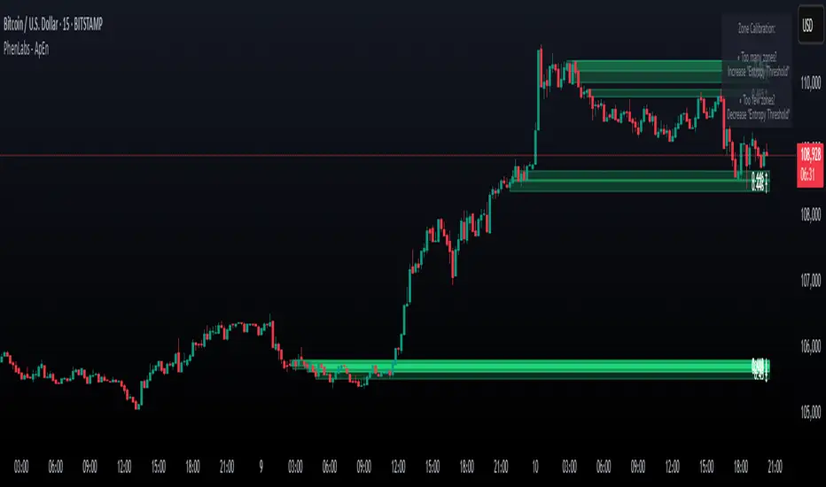
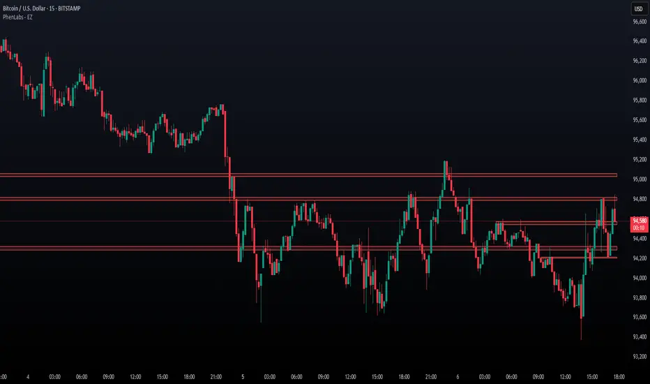
Approximate Entropy Zones [PhenLabs]Version: PineScript™ v6
Description
This indicator identifies periods of market complexity and randomness by calculating the Approximate Entropy (ApEn) of price action. As the movement of the market becomes complex, it means the current trend is losing steam and a reversal or consolidation is likely near. The indicator plots high-entropy periods as zones on your chart, providing a graphical suggestion to anticipate a potential market direction change. This indicator is designed to help traders identify favorable times to get in or out of a trade by highlighting when the market is in a state of disarray.
Points of Innovation
Advanced Complexity Analysis: Instead of relying on traditional momentum or trend indicators, this tool uses Approximate Entropy to quantify the unpredictability of price movements.
Dynamic Zone Creation: It automatically plots zones on the chart during periods of high entropy, providing a clear and intuitive visual guide.
Customizable Sensitivity: Users can fine-tune the ‘Entropy Threshold’ to adjust how frequently zones appear, allowing for calibration to different assets and timeframes.
Time-Based Zone Expiration: Zones can be set to expire after a specific time, keeping the chart clean and relevant.
Built-in Zone Size Filter: Excludes zones that form on excessively large candles, filtering out noise from extreme volatility events.
On-Chart Calibration Guide: A persistent note on the chart provides simple instructions for adjusting the entropy threshold, making it easy for users to optimize the indicator’s performance.
Core Components
Approximate Entropy (ApEn) Calculation: The core of the indicator, which measures the complexity or randomness of the price data.
Zone Plotting: Creates visual boxes on the chart when the calculated ApEn value exceeds a user-defined threshold.
Dynamic Zone Management: Manages the lifecycle of the zones, from creation to expiration, ensuring the chart remains uncluttered.
Customizable Settings: A comprehensive set of inputs that allow users to control the indicator’s sensitivity, appearance, and time-based behavior.
Key Features
Identifies Potential Reversals: The high-entropy zones can signal that a trend is nearing its end, giving traders an early warning.
Works on Any Timeframe: The indicator can be applied to any chart timeframe, from minutes to days.
Customizable Appearance: Users can change the color and transparency of the zones to match their chart’s theme.
Informative Labels: Each zone can display the calculated entropy value and the direction of the candle on which it formed.
Visualization
Entropy Zones: Shaded boxes that appear on the chart, highlighting candles with high complexity.
Zone Labels: Text within each zone that displays the ApEn value and a directional arrow (e.g., “0.525 ↑”).
Calibration Note: A small table in the top-right corner of the chart with instructions for adjusting the indicator’s sensitivity.
Usage Guidelines
Entropy Analysis
Source: The price data used for the ApEn calculation. (Default: close)
Lookback Length: The number of bars used in the ApEn calculation. (Default: 20, Range: 10-50)
Embedding Dimension (m): The length of patterns to be compared; a standard value for financial data. (Default: 2)
Tolerance Multiplier (r): Adjusts the tolerance for pattern matching; a larger value makes matching more lenient. (Default: 0.2)
Entropy Threshold: The ApEn value that must be exceeded to plot a zone. Increase this if too many zones appear; decrease it if too few appear. (Default: 0.525)
Time Settings
Analysis Timeframe: How long a zone remains on the chart after it forms. (Default: 1D)
Custom Period (Bars): The zone’s lifespan in bars if “Analysis Timeframe” is set to “Custom”. (Default: 1000)
Zone Settings
Zone Fill Color: The color of the entropy zones. (Default: #21f38a with 80% transparency)
Maximum Zone Size %: Filters out zones on candles that are larger than this percentage of their low price. (Default: 0.5)
Display Options
Show Entropy Label: Toggles the visibility of the text label inside each zone. (Default: true)
Label Text Position: The horizontal alignment of the text label. (Default: Right)
Show Calibration Note: Toggles the visibility of the calibration note in the corner of the chart. (Default: true)
Best Use Cases
Trend Reversal Trading: Identifying when a strong trend is likely to reverse or pause.
Breakout Confirmation: Using the absence of high entropy to confirm the strength of a breakout.
Ranging Market Identification: Periods of high entropy can indicate that a market is transitioning into a sideways or choppy phase.
Limitations
Not a Standalone Signal: This indicator should be used in conjunction with other forms of analysis to confirm trading signals.
Lagging Nature: Like all indicators based on historical data, ApEn is a lagging measure and does not predict future price movements with certainty.
Calibration Required: The effectiveness of the indicator is highly dependent on the “Entropy Threshold” setting, which needs to be adjusted for different assets and timeframes.
What Makes This Unique
Quantifies Complexity: It provides a numerical measure of market complexity, offering a different perspective than traditional indicators.
Clear Visual Cues: The zones make it easy to see when the market is in a state of high unpredictability.
User-Friendly Design: With features like the on-chart calibration note, the indicator is designed to be easy to use and optimize.
How It Works
Calculate Standard Deviation: The indicator first calculates the standard deviation of the source price data over a specified lookback period.
Calculate Phi: It then calculates a value called “phi” for two different pattern lengths (embedding dimensions ‘m’ and ‘m+1’). This involves comparing sequences of data points to see how many are “similar” within a certain tolerance (determined by the standard deviation and the ‘r’ multiplier).
Calculate ApEn: The Approximate Entropy is the difference between the two phi values. A higher ApEn value indicates greater irregularity and unpredictability in the data.
Plot Zones: If the calculated ApEn exceeds the user-defined ‘Entropy Threshold’, a zone is plotted on the chart.
Note: The “Entropy Threshold” is the most important setting to adjust. If you see too many zones, increase the threshold. If you see too few, decrease it.
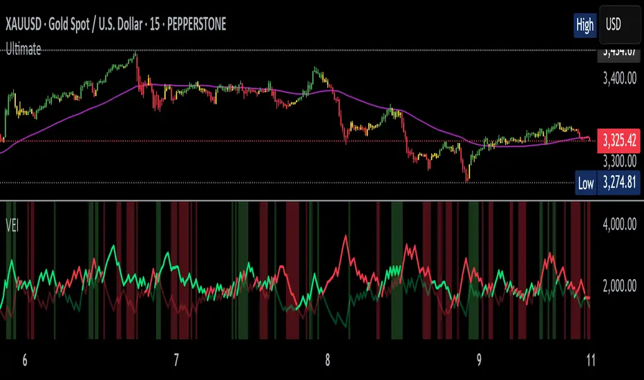
Volumetric Entropy IndexVolumetric Entropy Index (VEI)
A volume-based drift analyzer that captures directional pressure, trend agreement, and entropy structure using smoothed volume flows.
---
🧠 What It Does:
• Volume Drift EMAs : Shows buy/sell pressure momentum with adaptive smoothing.
• Dynamic Bands : Bollinger-style volatility wrappers react to expanding/contracting drift.
• Baseline Envelope : Clean structural white rails for mean-reversion zones or trend momentum.
• Background Shading : Highlights when both sides (up & down drift) are in agreement — green for bullish, red for bearish.
• Alerts Included : Drift alignment, crossover events, net drift shifts, and strength spikes.
---
🔍 What Makes It Different:
• Most volume indicators rely on bars, oscillators, or OBV-style accumulation — this doesn’t.
• It compares directional EMAs of raw volume to isolate real-time bias and acceleration.
• It visualizes the twisting tension between volume forces — not just price reaction.
• Designed to show when volatility is building inside the volume mechanics before price follows.
• Modular — every element is optional, so you can run it lean or fully loaded.
---
📊 How to Use It:
• Drift EMAs : Watch for one side consistently dominating — sharp spikes often precede breakouts.
• Bands : When they tighten and start expanding, it often signals directional momentum forming.
• Envelope Lines : Use as high-probability reversal or continuation zones. Bands crossing envelopes = potential thrust.
• Background Color : Green/red backgrounds confirm volume agreement. Can be used as a filter for other signals.
• Net Drift : Optional smoothed oscillator showing the difference between bullish and bearish volume pressure. Crosses above or below zero signal directional bias shifts.
• Drift Strength : Measures pressure buildup — spikes often correlate with large moves.
---
⚙️ Full Customization:
• Turn every layer on/off independently
• Modify all colors, transparencies, and line widths
• Adjust band width multiplier and envelope offset (%)
• Toggle bonus plots like drift strength and net baseline
---
🧪 Experimental Tools:
• Smoothed Net Drift trace
• Drift Strength signal
• Envelope lines and dynamic entropy bands with adjustable math
---
Built for signal refinement. Made to expose directional imbalance before the herd sees it.
Created by @Sherlock_Macgyver
Entropy Chart Analysis [PhenLabs]📊 Entropy Chart analysis -
Version: PineScript™ v6
📌 Description
The Entropy Chart indicator analysis applies Approximate Entropy (ApEn) to identify zones of potential support and resistance on your price chart. It is designed to locate changes in the market’s predictability, with a focus on zones near significant psychological price levels (e.g., multiples of 50). By quantifying entropy, the indicator aims to identify zones where price action might stabilize (potential support) or become randomized (potential resistance).
This tool automates the visualization of these key areas for traders, which may have the effect of revealing reversal levels or consolidation zones that would be hard to discern through traditional means. It also filters the signals by proximity to key levels in an attempt to reduce noise and highlight higher-probability setups. These dynamic zones adapt to changing market conditions by stretching, merging, and expiring based on user-inputted rules.
🚀 Points of Innovation
Combines Approximate Entropy (ApEn) calculation with price action near significant levels.
Filters zone signals based on proximity (in ticks) to predefined significant price levels (multiples of 50).
Dynamically merges overlapping or nearby zones to consolidate signals and reduce chart clutter.
Uses ApEn crossovers relative to its moving average as the core trigger mechanism.
Provides distinct visual coloring for bullish, bearish, and merged (mixed-signal) zones.
Offers comprehensive customization for entropy calculation, zone sensitivity, level filtering, and visual appearance.
🔧 Core Components
Approximate Entropy (ApEn) Calculation : Measures the regularity or randomness of price fluctuations over a specified window. Low ApEn suggests predictability, while high ApEn suggests randomness.
Zone Trigger Logic : Creates potential support zones when ApEn crosses below its average (indicating increasing predictability) and potential resistance zones when it crosses above (indicating increasing randomness).
Significant Level Filter : Validates zone triggers only if they occur within a user-defined tick distance from significant price levels (multiples of 50).
Dynamic Zone Management : Automatically creates, extends, merges nearby zones based on tick distance, and removes the oldest zones to maintain a maximum limit.
Zone Visualization : Draws and updates colored boxes on the chart to represent active support, resistance, or mixed zones.
🔥 Key Features
Entropy-Based S/R Detection : Uses ApEn to identify potential support (low entropy) and resistance (high entropy) areas.
Significant Level Filtering : Enhances signal quality by focusing on entropy changes near key psychological price points.
Automatic Zone Drawing & Merging : Visualizes zones dynamically, merging close signals for clearer interpretation.
Highly Customizable : Allows traders to adjust parameters for ApEn calculation, zone detection thresholds, level filter sensitivity, merging distance, and visual styles.
Integrated Alerts : Provides built-in alert conditions for the formation of new bullish or bearish zones near significant levels.
Clear Visual Output : Uses distinct, customizable colors for buy (support), sell (resistance), and mixed (merged) zones.
🎨 Visualization
Buy Zones : Represented by greenish boxes (default: #26a69a), indicating potential support areas formed during low entropy periods near significant levels.
Sell Zones : Represented by reddish boxes (default: #ef5350), indicating potential resistance areas formed during high entropy periods near significant levels.
Mixed Zones : Represented by bluish/purple boxes (default: #8894ff), formed when a buy zone and a sell zone merge, indicating areas of potential consolidation or conflict.
Dynamic Extension : Active zones are automatically extended to the right with each new bar.
📖 Usage Guidelines
Calculation Parameters
Window Length
Default: 15
Range: 10-100
Description: Lookback period for ApEn calculation. Shorter lengths are more responsive; longer lengths are smoother.
Embedding Dimension (m)
Default: 2
Range: 1-6
Description: Length of patterns compared in ApEn calculation. Higher values detect more complex patterns but require more data.
Tolerance (r)
Default: 0.5
Range: 0.1-1.0 (step 0.1)
Description: Sensitivity factor for pattern matching (as a multiple of standard deviation). Lower values require closer matches (more sensitive).
Zone Settings
Zone Lookback
Default: 5
Range: 5-50
Description: Lookback period for the moving average of ApEn used in threshold calculations.
Zone Threshold
Default: 0.5
Range: 0.5-3.0
Description: Multiplier for the ApEn average to set crossover trigger levels. Higher values require larger ApEn deviations to create zones.
Maximum Zones
Default: 5
Range: 1-10
Description: Maximum number of active zones displayed. The oldest zones are removed first when the limit is reached.
Zone Merge Distance (Ticks)
Default: 5
Range: 1-50
Description: Maximum distance in ticks for two separate zones to be merged into one.
Level Filter Settings
Tick Size
Default: 0.25
Description: The minimum price increment for the asset. Must be set correctly for the specific instrument to ensure accurate level filtering.
Max Ticks Distance from Levels
Default: 40
Description: Maximum allowed distance (in ticks) from a significant level (multiple of 50) for a zone trigger to be valid.
Visual Settings
Buy Zone Color : Default: color.new(#26a69a, 83). Sets the fill color for support zones.
Sell Zone Color : Default: color.new(#ef5350, 83). Sets the fill color for resistance zones.
Mixed Zone Color : Default: color.new(#8894ff, 83). Sets the fill color for merged zones.
Buy Border Color : Default: #26a69a. Sets the border color for support zones.
Sell Border Color : Default: #ef5350. Sets the border color for resistance zones.
Mixed Border Color : Default: color.new(#a288ff, 50). Sets the border color for mixed zones.
Border Width : Default: 1, Range: 1-3. Sets the thickness of zone borders.
✅ Best Use Cases
Identifying potential support/resistance near significant psychological price levels (e.g., $50, $100 increments).
Detecting potential market turning points or consolidation zones based on shifts in price predictability.
Filtering entries or exits by confirming signals occurring near significant levels identified by the indicator.
Adding context to other technical analysis approaches by highlighting entropy-derived zones.
⚠️ Limitations
Parameter Dependency : Indicator performance is sensitive to parameter settings ( Window Length , Tolerance , Zone Threshold , Max Ticks Distance ), which may need optimization for different assets and timeframes.
Volatility Sensitivity : High market volatility or erratic price action can affect ApEn calculations and potentially lead to less reliable zone signals.
Fixed Level Filter : The significant level filter is based on multiples of 50. While common, this may not capture all relevant levels for every asset or market condition. Accurate Tick Size input is essential.
Not Standalone : Should be used in conjunction with other analysis methods (price action, volume, other indicators) for confirmation, not as a sole basis for trading decisions.
💡 What Makes This Unique
Entropy + Level Context : Uniquely combines ApEn analysis with a specific filter for proximity to significant price levels (multiples of 50), adding locational context to entropy signals.
Intelligent Zone Merging : Automatically consolidates nearby buy/sell zones based on tick distance, simplifying visual analysis and highlighting stronger confluence areas.
Targeted Signal Generation : Focuses alerts and zone creation on specific market conditions (entropy shifts near key levels).
🔬 How It Works
Calculate Entropy : The script computes the Approximate Entropy (ApEn) of the closing prices over the defined Window Length to quantify price predictability.
Check Triggers : It monitors ApEn relative to its moving average. A crossunder below a calculated threshold (avg_apen / zone_threshold) indicates potential support; a crossover above (avg_apen * zone_threshold) indicates potential resistance.
Filter by Level : A potential zone trigger is confirmed only if the low (for support) or high (for resistance) of the trigger bar is within the Max Ticks Distance of a significant price level (multiple of 50).
Manage & Draw Zones : If a trigger is confirmed, a new zone box is created. The script checks for overlaps with existing zones within the Zone Merge Distance and merges them if necessary. Zones are extended forward, and the oldest are removed to respect the Maximum Zones limit. Active zones are drawn and updated on the chart.
💡 Note:
Crucially, set the Tick Size parameter correctly for your specific trading instrument in the “Level Filter Settings”. Incorrect Tick Size will make the significant level filter inaccurate.
Experiment with parameters, especially Window Length , Tolerance (r) , Zone Threshold , and Max Ticks Distance , to tailor the indicator’s sensitivity to your preferred asset and timeframe.
Always use this indicator as part of a comprehensive trading plan, incorporating risk management and seeking confirmation from other analysis techniques.
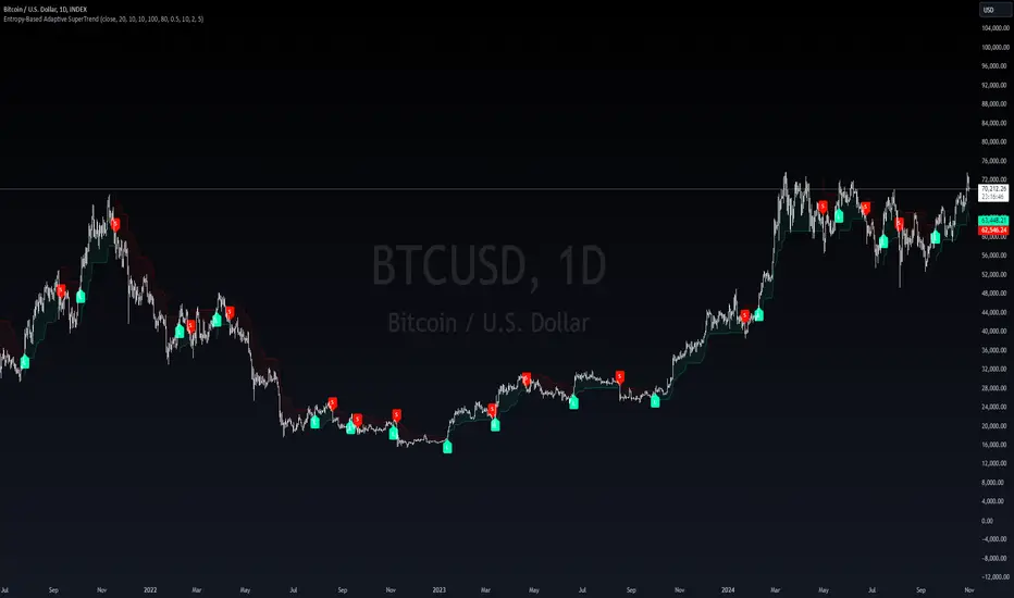
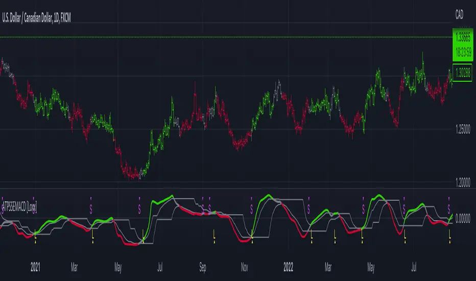
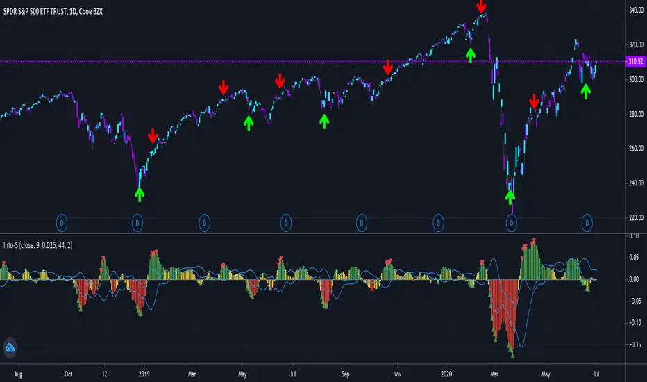
Entropy-Based Adaptive SuperTrendOverview:
Introducing the Entropy-Based Adaptive SuperTrend – a groundbreaking trading indicator designed to adapt dynamically to market conditions using market entropy. This enhanced SuperTrend indicator adjusts its sensitivity according to the level of chaos (or order) in price movements, providing more stable signals during volatile periods and more responsive signals when the market becomes orderly.
Key Features:
Entropy-Adaptive Mechanism: By incorporating an entropy measure, this indicator estimates the degree of unpredictability in the market. During high entropy periods (more chaotic), signals are made less sensitive, while during low entropy periods, the indicator reacts more quickly to price changes.
Adaptive ATR Multiplier: Unlike traditional SuperTrend indicators that use a fixed ATR multiplier, this version calculates a dynamic ATR multiplier based on the entropy score, ensuring more flexibility and adaptability in setting stop levels.
Visual Clarity: The indicator is overlayed on the price chart with customizable visual elements. The bullish and bearish trends are color-coded for ease of use, and optional entry signals ("L" for long and "S" for short) are plotted to clearly mark potential entry opportunities.
Alerts for Key Opportunities : Never miss an opportunity with built-in alerts for buy and sell signals. Traders can easily configure these alerts to be notified instantly when market conditions trigger a new trend.
How It Works:
Entropy Calculation: The entropy of the price data is calculated over a user-defined period, giving an indication of the degree of randomness in the price movements. The result is then smoothed to reduce noise and create a meaningful trend indication.
Dynamic ATR Adjustment: The ATR (Average True Range) multiplier, which controls the distance of the trailing stop, is adjusted based on the entropy score. This allows the SuperTrend line to widen in chaotic times, reducing false signals, while tightening in orderly times, allowing quicker trend captures.
Parameters Explained:
Entropy Settings: Control the sensitivity of entropy calculations, including the look-back period, number of bins for price distribution, and smoothing length.
Adaptive Settings: Adjust how the indicator adapts to different levels of entropy, including the adaptation period and the filtering weight.
SuperTrend Settings : Customize the ATR period and the dynamic multiplier range to fine-tune the trailing stops for your trading style.
Visual Settings: Choose your preferred colors for bullish and bearish trends, and decide if you want the entry labels displayed directly on the chart.
Use Cases:
Swing Traders can utilize the indicator to capture trend reversals while filtering out the noise during high entropy periods.
Intraday Traders can adapt the settings for shorter time frames to benefit from dynamic adjustments that reduce overtrading and false signals.
Risk Management: The entropy-based adaptive feature provides an edge in risk management by reducing sensitivity during times of increased chaos, thus helping to limit unnecessary trades.
How to Use It:
Look for entry labels ("L" for long, "S" for short) to identify potential opportunities.
Use the color-coded trendlines to determine market bias: greenish hue for bullish trends, reddish hue for bearish trends.
Customize the input settings to align with your preferred market timeframe and risk profile.
Alerts & Notifications:
Built-in alerts notify you of significant trend changes. Simply enable these alerts to receive updates when a new long or short opportunity is detected, helping you stay ahead without needing to watch the screen constantly.
Customization Tips:
Longer Timeframes : Increase the Entropy Period to better capture macro trends in high timeframe charts.
Higher Volatility Markets: Increase the ATR Max Multiplier to ensure stops are set farther away during high entropy.
Lower Volatility Markets: Use a lower ATR Base Multiplier and tighter entropy thresholds to capture rapid price movements.
Final Thoughts:
The Entropy-Based Adaptive SuperTrend indicator merges traditional trend-following logic with an adaptive mechanism driven by market entropy, aiming to address the challenges of whipsaws and false signals common in conventional SuperTrend setups. This indicator offers an intelligent and flexible way to track market trends, suitable for both beginners and experienced trade
Volume EntropyKey Components :
📍 Natural Logarithm Function : The script starts by employing a custom Taylor Series approximation for natural logarithms. This function serves to calculate entropy with higher accuracy than conventional methods, laying the foundation for further calculations.
📍 Entropy Calculation : The core of this indicator is its entropy function. It employs the custom natural log function to compute the randomness of the trading volume over a user-defined micro-pattern length, offering insights into market stability or volatility.
📍 Micro-Pattern Length : This is the parameter that sets the stage for the level of detail in the entropy calculation. Users can adjust it to suit different time frames or market conditions, thus customizing the indicator's sensitivity to randomness in trading volume.
Adaptive Two-Pole Super Smoother Entropy MACD [Loxx]Adaptive Two-Pole Super Smoother Entropy (Math) MACD is an Ehlers Two-Pole Super Smoother that is transformed into an MACD oscillator using entropy mathematics. Signals are generated using Discontinued Signal Lines.
What is Ehlers; Two-Pole Super Smoother?
From "Cycle Analytics for Traders Advanced Technical Trading Concepts" by John F. Ehlers
A SuperSmoother filter is used anytime a moving average of any type would otherwise be used, with the result that the SuperSmoother filter output would have substantially less lag for an equivalent amount of smoothing produced by the moving average. For example, a five-bar SMA has a cutoff period of approximately 10 bars and has two bars of lag. A SuperSmoother filter with a cutoff period of 10 bars has a lag a half bar larger than the two-pole modified Butterworth filter.Therefore, such a SuperSmoother filter has a maximum lag of approximately 1.5 bars and even less lag into the attenuation band of the filter. The differential in lag between moving average and SuperSmoother filter outputs becomes even larger when the cutoff periods are larger.
Market data contain noise, and removal of noise is the reason for using smoothing filters. In fact, market data contain several kinds of noise. I’ll group one kind of noise as systemic, caused by the random events of trades being exercised. A second kind of noise is aliasing noise, caused by the use of sampled data. Aliasing noise is the dominant term in the data for shorter cycle periods.
It is easy to think of market data as being a continuous waveform, but it is not. Using the closing price as representative for that bar constitutes one sample point. It doesn’t matter if you are using an average of the high and low instead of the close, you are still getting one sample per bar. Since sampled data is being used, there are some dSP aspects that must be considered. For example, the shortest analysis period that is possible (without aliasing)2 is a two-bar cycle.This is called the Nyquist frequency, 0.5 cycles per sample.A perfect two-bar sine wave cycle sampled at the peaks becomes a square wave due to sampling. However, sampling at the cycle peaks can- not be guaranteed, and the interference between the sampling frequency and the data frequency creates the aliasing noise.The noise is reduced as the data period is longer. For example, a four-bar cycle means there are four samples per cycle. Because there are more samples, the sampled data are a better replica of the sine wave component. The replica is better yet for an eight-bar data component.The improved fidelity of the sampled data means the aliasing noise is reduced at longer and longer cycle periods.The rate of reduction is 6 dB per octave. My experience is that the systemic noise rarely is more than 10 dB below the level of cyclic information, so that we create two conditions for effective smoothing of aliasing noise:
1. It is difficult to use cycle periods shorter that two octaves below the Nyquist frequency.That is, an eight-bar cycle component has a quantization noise level 12 dB below the noise level at the Nyquist frequency. longer cycle components therefore have a systemic noise level that exceeds the aliasing noise level.
2. A smoothing filter should have sufficient selectivity to reduce aliasing noise below the systemic noise level. Since aliasing noise increases at the rate of 6 dB per octave above a selected filter cutoff frequency and since the SuperSmoother attenuation rate is 12 dB per octave, the Super- Smoother filter is an effective tool to virtually eliminate aliasing noise in the output signal.
What are DSL Discontinued Signal Line?
A lot of indicators are using signal lines in order to determine the trend (or some desired state of the indicator) easier. The idea of the signal line is easy : comparing the value to it's smoothed (slightly lagging) state, the idea of current momentum/state is made.
Discontinued signal line is inheriting that simple signal line idea and it is extending it : instead of having one signal line, more lines depending on the current value of the indicator.
"Signal" line is calculated the following way :
When a certain level is crossed into the desired direction, the EMA of that value is calculated for the desired signal line
When that level is crossed into the opposite direction, the previous "signal" line value is simply "inherited" and it becomes a kind of a level
This way it becomes a combination of signal lines and levels that are trying to combine both the good from both methods.
In simple terms, DSL uses the concept of a signal line and betters it by inheriting the previous signal line's value & makes it a level.
Included:
Bar coloring
Alerts
Signals
Loxx's Expanded Source Types
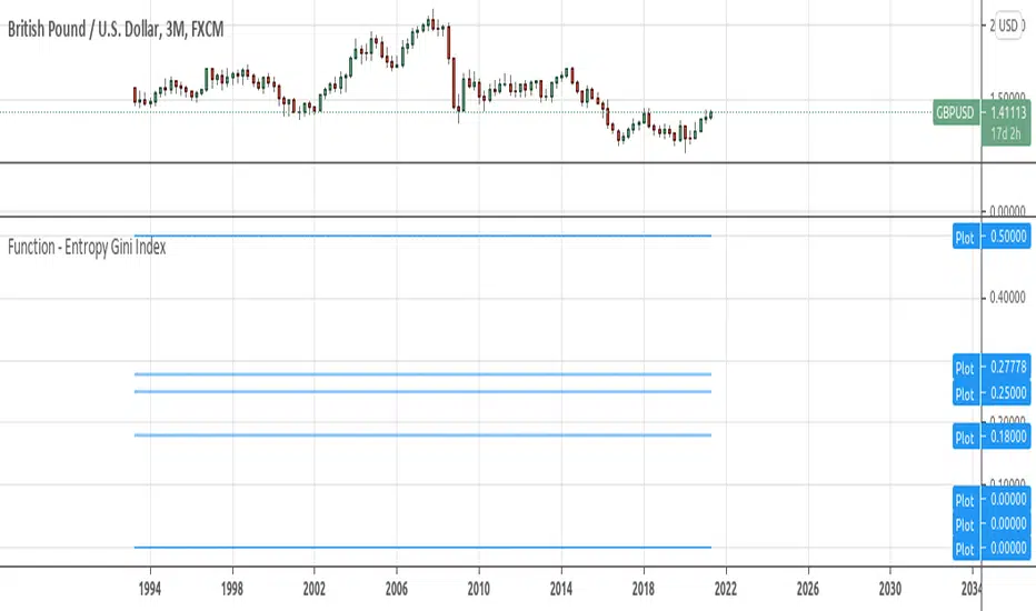
Basic Shannon Entropy & DerivativesThis script performs the basic Shannon entropy on the closing value of the stock. Additionally, it performs the trailing first and second derivatives of the Shannon Entropy, giving you more information about its movement.
You can change the "Source" to be whatever value you like.
ProbabilityLibrary "Probability"
erf(value) Complementary error function
Parameters:
value : float, value to test.
Returns: float
ierf_mcgiles(value) Computes the inverse error function using the Mc Giles method, sacrifices accuracy for speed.
Parameters:
value : float, -1.0 >= _value >= 1.0 range, value to test.
Returns: float
ierf_double(value) computes the inverse error function using the Newton method with double refinement.
Parameters:
value : float, -1. > _value > 1. range, _value to test.
Returns: float
ierf(value) computes the inverse error function using the Newton method.
Parameters:
value : float, -1. > _value > 1. range, _value to test.
Returns: float
complement(probability) probability that the event will not occur.
Parameters:
probability : float, 0 >=_p >= 1, probability of event.
Returns: float
entropy_gini_impurity_single(probability) Gini Inbalance or Gini index for a given probability.
Parameters:
probability : float, 0>=x>=1, probability of event.
Returns: float
entropy_gini_impurity(events) Gini Inbalance or Gini index for a series of events.
Parameters:
events : float , 0>=x>=1, array with event probability's.
Returns: float
entropy_shannon_single(probability) Entropy information value of the probability of a single event.
Parameters:
probability : float, 0>=x>=1, probability value.
Returns: float, value as bits of information.
entropy_shannon(events) Entropy information value of a distribution of events.
Parameters:
events : float , 0>=x>=1, array with probability's.
Returns: float
inequality_chebyshev(n_stdeviations) Calculates Chebyshev Inequality.
Parameters:
n_stdeviations : float, positive over or equal to 1.0
Returns: float
inequality_chebyshev_distribution(mean, std) Calculates Chebyshev Inequality.
Parameters:
mean : float, mean of a distribution
std : float, standard deviation of a distribution
Returns: float
inequality_chebyshev_sample(data_sample) Calculates Chebyshev Inequality for a array of values.
Parameters:
data_sample : float , array of numbers.
Returns: float
intersection_of_independent_events(events) Probability that all arguments will happen when neither outcome
is affected by the other (accepts 1 or more arguments)
Parameters:
events : float , 0 >= _p >= 1, list of event probabilities.
Returns: float
union_of_independent_events(events) Probability that either one of the arguments will happen when neither outcome
is affected by the other (accepts 1 or more arguments)
Parameters:
events : float , 0 >= _p >= 1, list of event probabilities.
Returns: float
mass_function(sample, n_bins) Probabilities for each bin in the range of sample.
Parameters:
sample : float , samples to pool probabilities.
n_bins : int, number of bins to split the range
@return float
cumulative_distribution_function(mean, stdev, value) Use the CDF to determine the probability that a random observation
that is taken from the population will be less than or equal to a certain value.
Or returns the area of probability for a known value in a normal distribution.
Parameters:
mean : float, samples to pool probabilities.
stdev : float, number of bins to split the range
value : float, limit at which to stop.
Returns: float
transition_matrix(distribution) Transition matrix for the suplied distribution.
Parameters:
distribution : float , array with probability distribution. ex:.
Returns: float
diffusion_matrix(transition_matrix, dimension, target_step) Probability of reaching target_state at target_step after starting from start_state
Parameters:
transition_matrix : float , "pseudo2d" probability transition matrix.
dimension : int, size of the matrix dimension.
target_step : number of steps to find probability.
Returns: float
state_at_time(transition_matrix, dimension, start_state, target_state, target_step) Probability of reaching target_state at target_step after starting from start_state
Parameters:
transition_matrix : float , "pseudo2d" probability transition matrix.
dimension : int, size of the matrix dimension.
start_state : state at which to start.
target_state : state to find probability.
target_step : number of steps to find probability.
Function - Entropy Gini Indexfunction to retrieve Gini Impurity / Gini Index.
reference:
- victorzhou.com
- en.wikipedia.org
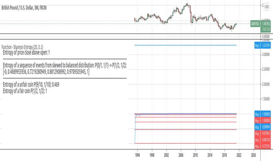
Function - Shannon Entropyfunctions for shannon's entropy
reference:
- en.wiktionary.org
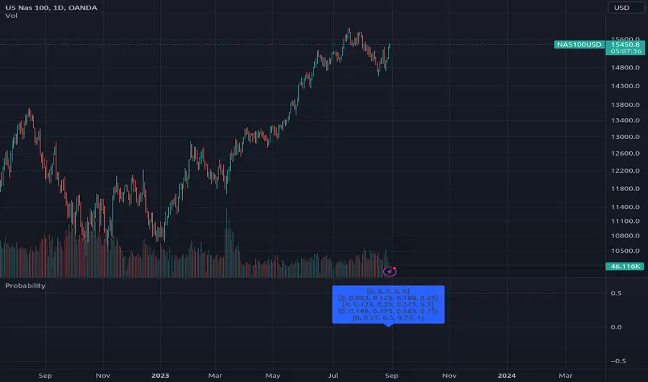
- machinelearningmastery.com
Bernoulli Process - Binary Entropy FunctionThis indicator is the Bernoulli Process or Wikipedia - Binary Entropy Function . Within Information Theory, Entropy is the measure of available information, here we use a binary variable 0 or 1 (P) and (1-P) (Bernoulli Function/Distribution), and combined with the Shannon Entropy measurement. As you can see below, it produces some wonderful charts and signals, using price, volume, or both summed together. The chart below shows you a couple of options and some critical details on the indicator. The best part about this is the simplicity, all of this information in a couple of lines of code.
Using the indicator:
The longer the Entropy measurement the more information you are capturing, so the analogy is, the shorter the signal, the less information you have available to utilize. You'll run into your Nyquist frequencies below a length of 5. I've found values between 9 and 22 work well to gather enough measurements. You also have an averaging summation that measures the weight or importance of the information over the summation period. This is also used for highlighting when you have an information signal above the 5% level (2 sigma) and then can be adjusted using the Percent Rank Variable. Finally, you can plot the individual signals (Price or Volume) to get another set of measurements to utilize. As can be seen in the chart below, the volume moves before price (but hopefully you already knew that)
At its core, this is taking the Binary Entropy measurement (using a Bernoulli distribution) for price and volume. I've subtracted the volume from the price so that you can use it like a MACD, also for shorter time frames (7, 9, 11) you can get divergences on the histogram. These divergences are primarily due to the weekly nature of the markets (5 days, 10 days is two weeks,...so 9 is measuring the last day of the past two weeks...so 11 is measuring the current day and the past two weeks).
Here are a couple of other examples, assuming you just love BTC, Stocks, or FOREX. I fashioned up a strategy to show the potential of the indicator.
BTC-Strategy
Stock-Strategy (#loveyouNFLX)
FOREX - (for everyone hopped up on 40X leverage)

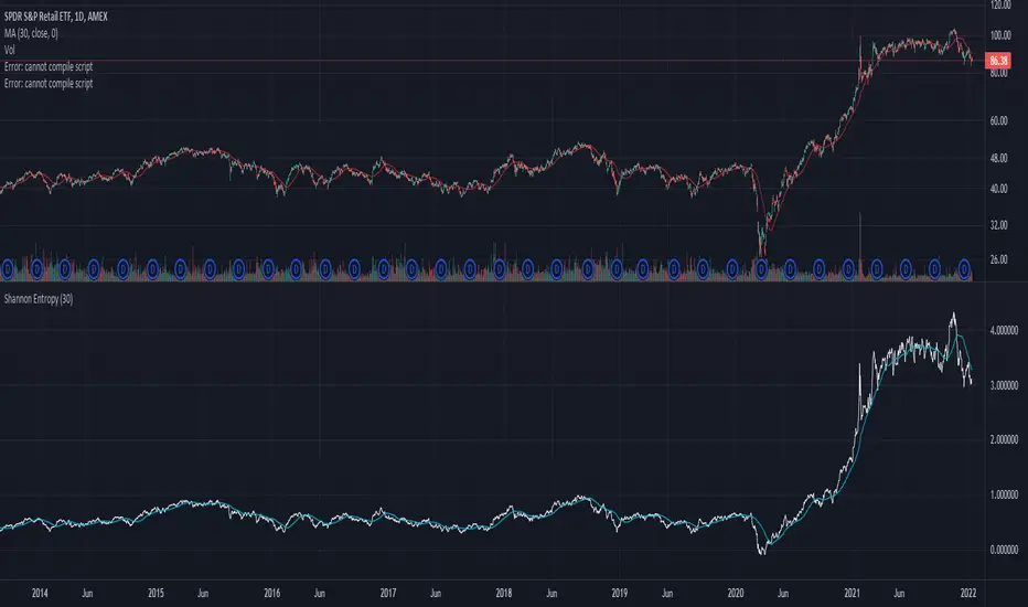
Shannon Entropy V2Version 2, Shannon Entropy
This update includes both a deadband (Plotting Optional) and PercentRank Indicating.
Here is a unique way of looking at your price & volume information. Utilize the calculated value of "Shannon Entropy". This is a measure of "surprise" in the data, the larger the move or deviation from the most probable value, the higher the new information gain. What I think is so interesting about this value, is the smoothness that it displays the information without using moving averages. There is a lot of meat on this bone to be incorporated in other scripts.
H = -sum(prob(i) * log_base2(prob(i)))
I've included the typical way that I've been experimenting with this, which is the difference between the volume information and price information. I've included the option to turn either price or volume data off to see the Shannon Entropy value of either value. There are a ton of complex scripts out there trying to do what this calculation is doing in 3 lines. As with anything, there are no free lunches, so you can nicely see as you lower the lengths you'll quickly learn where your nyquist frequencies are at, you'll want to work at about double the noisy value at a minimum.
Using this script is based on "Information" and it highlights places that need your attention, either because there is a large amount of change (new information) or there is minimal new information (complacency, institutional movements). Buy and Sell points are up to the user, this is just showing you where you need to provide some attention.
You can use it with or without volume data, you can also isolate either the source and volume. Below are some options for printing:
It can also with BTC (better with volume data)
Big shoutout to yatrader2 for great Shannon Entropy discussions.
And to Picte/ for his interesting inspiration STOCH-HVP-picte
Shannon EntropyHere is a unique way of looking at your price & volume information. Utilize the calculated value of "Shannon Entropy". This is a measure of "surprise" in the data, the larger the move or deviation from the most probable value, the higher the new information gain. What I think is so interesting about this value, is the smoothness that it displays the information without using moving averages. There is a lot of meat on this bone to be incorporated in other scripts.
H = -sum(prob(i) * log_base2(prob(i)))
I've included the typical way that I've been experimenting with this, which is the difference between the volume information and price information. I've included the option to turn either price or volume data off to see the Shannon Entropy value of either value. There are a ton of complex scripts out there trying to do what this calculation is doing in 3 lines.
As with anything, there are no free lunches, so you can nicely see as you lower the lengths you'll quickly learn where your nyquist frequencies are at, you'll want to work at about double the noisy value at a minimum.
